Introduction

Tensors and their contraction

Tensor is a higher-dimensional generalization of the matrix, which has two indices such as $M_{ij}$. For example, a four-dimensional tensor can be obtained by the tensor product of two matrices $\left(A\otimes B\right)\_{ij}=C_{ij}=C_{k\cdot d_{l}+l, m\cdot d_{n}+n}=A_{km}\cdot B_{ln}\equiv T_{mn}^{kl}$, where $d_{l, n}$ are the dimensions of the corresponding indices. Each index of a tensor is called a bond. Any element in a rank-$D$ tensor $T_{n_{0}, n_{1}, \cdots, n_{D-1}}$ can be mapped to a one-dimensional vector $v(p)$, which is the actual physical storage in a computer's memory. Generally there are two ways to do this.

Row-major. $p=\sum_{k=0}^{D-1}n_{k}\cdot\left(\prod_{l=k+1}^{D-1}d_{l}\right)$. The elements along the last index are contiguous. It is implemented in numpy as default.
Column-major. $p=\sum_{k=0}^{D-1}n_{k}\cdot\left(\prod_{l=0}^{k-1}d_{l}\right)$. The elements along the first index are contiguous. It is implemented in Fortran and Eigen::Tensor<> (C++) as default.

Two different tensors can be contracted if they share a same dimension. It is a generalization of the matrix production like $C_{ij}=\sum_{k}A_{ik}B_{kj}$. Graphically, we use a connected link to denote the connection of two bonds. Tensors with some connected and unconnected bonds can form a tensor network (TN).

Matrix product state and matrix product operator

Firstly I should point out the so-called and matrix product operator (MPO) are actually comprised of tensors rather than matrices. This is a historical issue. A one-dimensional (1D) quantum state can be written as a matrix product state (MPS):

$$ \begin{equation} |\psi\rangle=\sum_{\{j\}}\left(A^{j_{0}}\cdots A^{j_{N-1}}\right)|j_{0}\cdots j_{N-1}\rangle. \end{equation} $$

$A$ has already been chosen to be left-canonical, namely $\sum_{j}A^{j\dagger}A^{j}=1$. The basic idea of MPO is to introduce more inner bonds to decouple the operation of a many-body operator with finite range interactions into the production of local onsite tensors.

A matrix product operator (MPO) looks like

$$ \begin{equation} H=W_{\gamma_{0}\gamma_{1}}^{j_{0}^{\prime}j_{0}}W_{\gamma_{1}\gamma_{2}}^{j_{1}^{\prime}j_{1}}\cdots W_{\gamma_{N-1}\gamma_{0}}^{j_{N-1}^{\prime}j_{N-1}}|\{j^{\prime}\}\rangle\langle\{j\}|. \end{equation} $$

$\gamma_{0}=1$ denotes a virtual bond.

One of the simplest physical TN is to compute the expectation value of a MPO in terms a MPS like $\langle\psi|H|\psi\rangle$, which can be expressed as

TN representation for $\langle\psi|H|\psi\rangle$.

How to practically contract a TN

An example

Here we consider a TN $\langle\psi|H|\psi\rangle$ as an example, in which $H$ is chosen to be the XYZ-model

$$ \begin{equation} H=\sum_{j=0}^{N-2}\left(J_{x}\sigma_{j}^{x}\sigma_{j+1}^{x}+J_{y}\sigma_{j}^{y}\sigma_{j+1}^{y}+J_{z}\sigma_{j}^{z}\sigma_{j+1}^{z}\right)+h\sum_{j=0}^{N-1}\sigma_{j}^{z}. \end{equation} $$

Written into a MPO

$$ \begin{equation} W_{n}= \begin{pmatrix} 1 & 0 & 0 & 0 & 0 \\ J_{x}\sigma^{x} & 0 & 0 & 0 & 0 \\ J_{y}\sigma^{y} & 0 & 0 & 0 & 0 \\ J_{z}\sigma^{z} & 0 & 0 & 0 & 0 \\ h\sigma^{z} & \sigma^{x} & \sigma^{y} & \sigma^{z} & 1 \end{pmatrix}. \label{eq:bulk_mpo} \end{equation} $$

we have several methods to contract this TN:

Naive method (NM). By a naive way, we can paste all the tensors piece by piece utilizing numpy.tensordot. On site $j$, we can paste the upper MPS, MPO and lower mps into a rank-6 onsite tensor. Then paste it to the environment tensor, which has three virtual bonds. As a member function of the MPO, it looks like:
Optimized einsum (OE). By utilizing opt_einsum¹, we can speed up the contraction dramatically, which could find the optimal contraction order automatically. At each site $j$, we can contract the environment, upper MPS, MPO and lower MPS at the same time. Moreover, it supports CUDA through CuPy.
Optimized einsum as a whole graph. Instead of site by site, we can pass all the tensors and contracting information to opt_einsum, which can handle the whole TN and find out the optimal contracting path. This method will be particularly useful to contracting a two-dimensional TN.

Numerical results

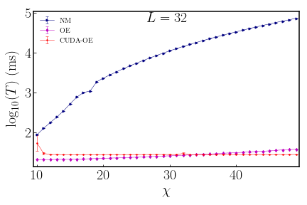
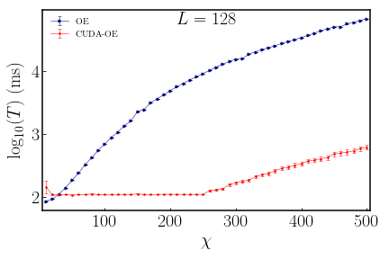
Platform: Intel(R) Xeon(R) CPU E5-2640, NVIDIA Tesla P100, CUDA 9.2.88. The XYZ-Hamiltonian is chosen as $J_{x}=J_{y}=1.0, J_{z}=h=0.5$. The MPS is generated randomly.

We conclude that:

By utilizing opt_einsum in stead of the naive tensordot, the contraction can be dramatically speeded up $10^{3}$ times as much as possible especially with large bond dimension $\chi$. With relatively small $\chi$, CUDA-OE is even slower than OE, while not too much.
CUDA can further speed up about as many as $10^{2}$ times. It reaches the threshold at about $\chi\simeq 250$, below which we think that the cores in GPU are not fully implemented. Overall, if we use opt_einsum combined with CUDA, we can speed up the tensor contraction as many as $10^{5}$ times in comparison with the naive tensordot.

Time for contracting a TN in terms of NM, OE and CUDA-OE.

Time for contracting a TN in terms of OE and CUDA-OE.

The original notebook and code can be found here.

Smith et al., (2018). opt_einsum - A Python package for optimizing contraction order for einsum-like expressions . Journal of Open Source Software, 3(26), 753. ↩