Matrix multiplication and tensor contraction cost

The computational cost of a matrix multiplication $A\cdot{B}$ reads $\mathfrak{C}\left(A\cdot{B}\right)=d_{0}d_{1}d_{2}$ with $A$ is a $d_{0}\times{d}_{1}$ matrix and $B$ is a $d_{1}\times{d}_{2}$ matrix, which means typically the computer needs to perform $\left(d_{0}d_{1}d_{2}\right)$ times floating point multiplication. Similarly, if $A$ and $B$ are generalized tensors as in FIG. 1(b), the corresponding tensordot cost is¹

$$ \begin{equation} \mathfrak{C}\left(A\cdot{B}\right)=d^{3}d^{2}=\frac{|\text{dim}(A)|\cdot|\text{dim}(B)|}{|\text{dim}(A\cap{B})|}, \end{equation} $$

since we need to sum over two internal connected indices at the same time.

FIG. 1. Matrix mutiplication and tensor contractions.

If a network consisting of more than two tensors is considered such as FIG. 1(c), one can contract the inner connected indices at the same time, which leads to a $d^{4}$ cost. Alternatively, we can contract them iteratively tensor by tensor, which leads to a cost $\mathfrak{C}((A\cdot{B})\cdot{C})=2d^{3}$. If $d>2$, the later way is more efficient.

An example in DMRG

If we choose to contract a TN iteratively tensor by tensor, then we have different paths, which turn out to have different costs. An example can be shown in the variational matrix product state method, where we need to solve the linear eigen-problem

$$ \begin{equation} \mathcal{H}A=\lambda{A} \end{equation} $$

involving the effective Hamiltonian $\mathcal{H}$ contracting from the environment tensors $L$, $R$ and the MPO tensor $W$. $A$ is the one-site MPS tensor. We prefer to use the iterative method such as Lanczos. The major cost during this process is the generalized "matrix multiplication", namely the contraction of $L, W, R, A$ as shown in FIG. 2(a). $\chi$ is the bond dimension of the virtual bond in the MPS, $D$ is the MPO's bond dimension and $d$ is the physical bond dimension. $d=2$ for spin-$1/2$ systems. Typically, $\chi\gg{D}>d$.

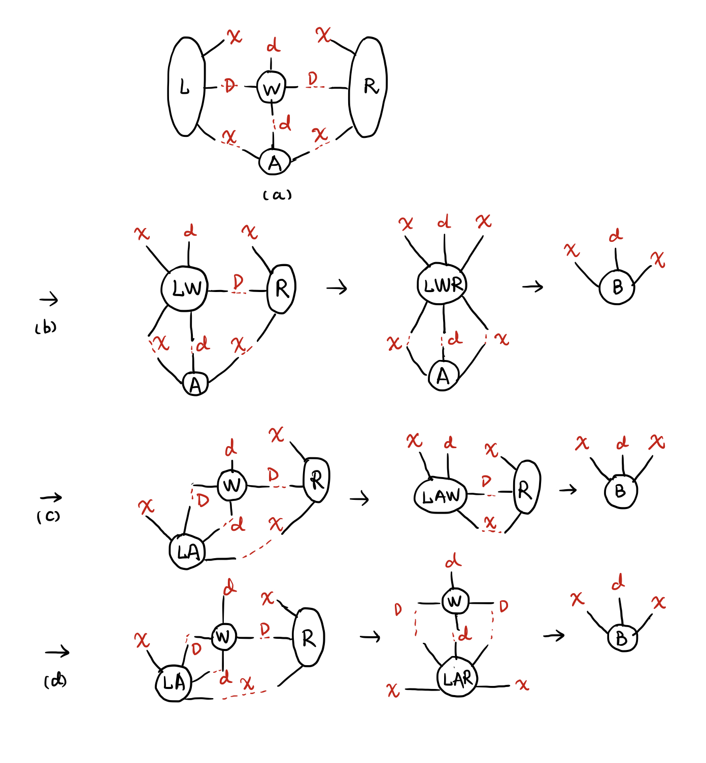
FIG. 1. Matrix mutiplication and tensor contractions.

Thus, we have different paths to contract. As shown in FIG. 2(b, c, d), we have

$$ \begin{align} \mathfrak{C}_{b}({L}\cdot{W}\cdot{R}\cdot{A})&=\chi^{2}D^{2}d^{2}+\chi^{4}Dd^{2}+\chi^{4}d^{2}, \\ \mathfrak{C}_{c}({L}\cdot{A}\cdot{W}\cdot{R})&=2\chi^{3}Dd+\chi^{2}D^{2}d^{2}, \\ \mathfrak{C}_{d}({L}\cdot{A}\cdot{R}\cdot{W})&=\chi^{3}Dd+\chi^{3}D^{2}d+\chi^{2}D^{2}d^{2}. \end{align} $$

Obviously, FIG. 2(c) is the optimal path if $\chi$ is much larger than $D$ and $d$, which is can be automatically found by opt_einsum². opt_einsum is tested to be as fast as numpy.tensordot with the same path.